Getting Started

This document is intended as starting point for wingstructure usage. The wingstructure package has three main features:

• representation of wing geometry

  Hereby the representation of a wing geometry in yaml files and a object oriented representation in python is ment.

• calculation of lift distribution

  The distribution of lift and aerodynamic moments can be calculated using multhopps quadrature method.

• estimation of wing structure mass and structural analysis (sectionwise)

  Starting from an airfoil dat file various structure elements (shell, spar) can be added. The mass and some structural quantities can be calculated.

A brief introduction for those functions is given in this document. For more detailed information have a look at the Jupyter notebook examples. Some topics are already covered by specific documenatation pages in deeper detail. Those are linked within the following sections.

Installation

Before wingstructure can be used, it has to be installed. This can be done with pip:

pip install https://github.com/akafliegdarmstadt/wingstructure/archive/master.zip

Basic examples

Creating a wing

wingstructure can read geometry definition from yaml files, which simplifies the reuse of those definitions in multiple scripts. The wing of D-38 can be described with the following yaml file:

D-38.yaml

geometry:
  wing:
    sections:
    - pos:
          x: 0.0
          y: 0.0
          z: 0.0
      chord: 0.943
      airfoil: 'FX 61-184'
    - pos:
          y: 4.5
      chord: 0.754
      twist: -1.13
      airfoil: 'FX 61-184'
    - pos:
          x: 0.134
          y: 7.5
      chord: 0.377
      twist: -3.86
      airfoil: 'FX 60-126'
    control-surfaces:
      QR:
        type: 'aileron'
        span-start: 4.125
        span-end: 7.125
        chord-pos: 0.8
      BK:
        type: 'spoiler'
        span-start: 2.035
        span-end: 3.310
        chord-pos: 0.6

To make the document extensible the wing geometry is stored inside of a wing object, which itself is placed within geometry. Starting with line 3 the wing planform is defined through sections. The content should be rather self explanatory.

After the sections control surfaces are defined.

This definition can be loaded with any yaml parser, but it is recommended to use wingstructure’s wingstructure.data.loaddata() function:

In [1]: from wingstructure import data

In [2]: definition = data.loaddata('usage/D-38.yaml')

For a more convenient access to the data an wingstructure.data.Wing object is created.

In [3]: wing = data.Wing.create_from_dict(definition['geometry']['wing'])

In [4]: wing.plot()

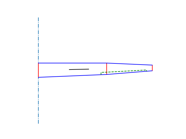
Besides plotting the wing object has some useful properties. For example calculating the mean aerodynamic chord:

In [5]: wing.mac
Out[5]: sec: {leading edge: Point(x=0.018321048098281882, y=3.294505643954848, z=0.0), chord: 0.7703129788295028}

Further information can be found in wingstructure.data.Wing.

Calculating wing’s lift distribution

The wing is now defined and can be analysed. Therefore the analysis submodule of wingstructure is imported. Within this submodule you find an LiftAnalyis class, which will be used now.

In [6]: from wingstructure.aero import analysis

In [7]: liftana = analysis.LiftAnalysis(wing)

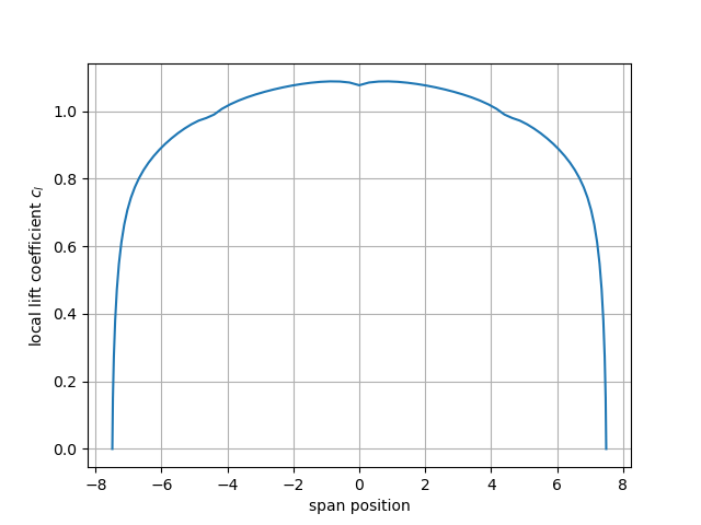
In [8]: alpha, c_ls = liftana.calculate(1.0)

This calculates the angle of attack and local lift coefficients. Those are plotted in the following. The associated span positions are stored inside liftana (wingstructure.analysis.LiftAnalysis.calc_ys).

In [9]: from matplotlib import pyplot as plt

In [10]: plt.figure();

In [11]: plt.plot(liftana.calc_ys, c_ls)
   ....: plt.xlabel('span position')
   ....: plt.ylabel('local lift coefficient $c_l$')
   ....: plt.grid();
   ....: 

With creation of liftana automatically distributions for all control surfaces are created. The method wingstructure.analysis.LiftAnalysis.calculate() combines those to calculate local lift coefficient and angle of attack for a requested lift. Its parameters allow also the enabling of spoilers and deflection of other control surfaces. Have a look at this analysis and the documentation wingstructure.analysis.calculate().

Estimating wing section’s mass

Calculating the mass of a wing section is not that closely connected to the previous freatures. You start with the import of the wingstructure.structure module and loading of an airfoil dat file. For loading numpy.loadtxt() is used.

In [12]: from wingstructure import structure

In [13]: import numpy as np

In [14]: coords = np.loadtxt('usage/FX 61-184.dat', skiprows=1, delimiter=',')

The loaded airfoil file can for examle be found here

To analyse a section with this airfoil as outline an instance of wingstructure.structure.SectionBase is created.

In [15]: secbase = structure.SectionBase(coords)

Before filling this outline with structure we define a material:

In [16]: import collections as col

In [17]: Material = col.namedtuple('Material', ['ρ'])

In [18]: basematerial = Material(ρ=0.3e3)

Now the structure can be created. Definition begins from the outside inwards. First feature is a constant layer (for example a fabric). We continue with a spar definition and analyse the section’s mass.

In [19]: layer = structure.Layer(basematerial, 3e-3)

In [20]: spar = structure.ISpar({'flange': basematerial,
   ....:                         'web': basematerial},
   ....:                          0.5,
   ....:                        0.300,
   ....:                        3e-2,
   ....:                        0.8,
   ....:                        1e-3)
   ....: secbase.extend([layer, spar])
   ....: 

In [21]: massana = structure.MassAnalysis(secbase)
   ....: massana.massproperties
   ....: 
Out[21]: (array([0.49549871, 0.02784994]), 7.231461694880079)

For a more complex example have a look at the corresponding notebook .